关于微信公众号

咕了快半年233333

这里是RSA最最基础的，也是最最常规的利用，都是由于对算法的不正确使用而造成的，coppersmith相关的attack请移步密码学学习笔记 之 Coppersmith’s Method

解密算法正确性的证明

首先从解密算法的正确性证明起手，即证明$m \equiv c^d \pmod n$

欧拉定理：若$a,n$为正整数，且$𝑎,𝑛$互素（即$gcd(a,n) = 1$），则$𝑎^{𝜑(𝑛)} \equiv 1 \pmod n$。
已知 $1 \equiv e\cdot d \pmod {φ(n)}，𝑚 < 𝑛，c \equiv m^e \pmod n，gcd(𝑚,𝑛) = 1$，求证$m \equiv c^d \pmod n$

等式左边为m

等式右边为$c^d \pmod{n}$
∵ $𝑐 \equiv m^e\pmod n $$

∴ $c^d \pmod n \equiv (m^e \pmod n)^d \pmod n \equiv m^{e\cdot d} \pmod n $

∵ $1 \equiv e\cdot d \pmod {φ(n)} $

∴ $e\cdot d \equiv k\cdot φ(n) + 1 $

∴ $c^d \equiv m^{e \cdot d} \equiv m^{k\cdot φ(n)+1} \equiv m\cdot (m^{φ(n)})^k \pmod n $

∵ $gcd(m,n) \equiv 1$

∴ $m^{φ(n)} \equiv 1 \pmod n $

∴ $c^d \equiv m\cdot (m^{φ(n)})^k \equiv m\cdot (1)^k \equiv m \pmod n $

∵ $m<n$

∴ $m \pmod n \equiv m$

∴ $c^d \equiv m \pmod n \equiv m $

等式右边等于等式左边，证毕。

---

p和q相差过小

如果题目代码给到$p = nextprime(q)$这样

那么说明$p$和$q$特别接近，所以可以看作$n = p^2$

所以我们直接对$n$开方就可以得到$p、q$之间的一个值$t$，进而求一个$nextprime(t)$即可得到$p$

模n有公约数

利用欧几里得辗转相除法（$gcd$）即可得到$n$的公约数

已知e,d,n分解模求p,q

原理来自这篇综述

给定$d$，计算$k=d\cdot e−1$。根据$d$和$e$的定义我们知道$k$是$φ(N)$的倍数。由于$φ(N)$是偶数，$k=2^tr$其中$r$为奇数且$t≥1$。对于每个$g\in \mathbb{Z_n}$都有$g^k=1$，因此$g^{\frac{k}{2}}$是单位模$N$的平方根。根据中国剩余定理，1在模$N$下有四个平方根。其中两个平方根是$±1$，另外两个是$±x$，其中x满足$x\equiv 1 \pmod p$和$x\equiv −1 \pmod q$。用这最后两个平方根中的任意一个，通过计算$gcd(x−1,N)$来揭示$N$的因式分解。一个直截了当的论证表明，如果从$\mathbb{Z_n}$中随机选择$g$，那么序列中的一个元素$g^{\frac{k}{2}}，g^{\frac{k}{4}},…，g^{\frac{k}{2^t}} \pmod N$是统一平方根的概率至少为$\frac{1}{2}$，从而揭示了$N$的分解，序列中的所有元素可以在时间$\mathcal{O}(n^3))$内有效地计算，其中$n=log_2N$。

from gmpy2 import gcd
from random import *
  
def factor_n_with_ed(n,e,d):  
    p = 1  
    q = 1  
    while p==1 and q==1:  
        k = d * e - 1  
        g = random.randint ( 0 , n )  
        while p==1 and q==1 and k % 2 == 0:  
            k /= 2  
            y = pow(g,k,n)  
            if y!=1 and gcd(y-1,n)>1:  
                p = gcd(y-1,n)  
                q = n/p  
    return p,q

$d_p、d_q$泄露

摘自这篇私钥重构

首先说明$d_p$和$d_q$的含义

$d_p \equiv d \pmod{φ(p)}$
$d_q \equiv d \pmod{φ(q)}$

利用条件：已知$p，q，d_p，d_q，c$，无公钥$e$、私钥$d$

证：

由 $e\cdot d \equiv 1 \pmod {(p-1)\cdot (q-1)}$

​ $d_p \equiv d \pmod{φ(p)}$

得 $e\cdot d_p \equiv 1 \pmod {φ(p)} $

设$m_1 \equiv m^{e\cdot d_p} \equiv c^{d_p} \pmod p$

则$m_1 \equiv m^{k\cdot φ(p)+1} \pmod p $

由费马小定理，$m^{φ(p)} \equiv 1 \pmod p$

所以$ m_1 \equiv m \pmod p$

同理 $m_2 \equiv m \equiv c^{d_q} \pmod q$

然后我们就有同余式方程组：$m \equiv m_1 \pmod p$

​ $m \equiv m_2 \pmod q$

然后走一波CRT恢复$m$就好了（$m < p\cdot q$）

exp:

mp = pow(c,dp,p)
mq = pow(c,dq,q)
a = invert(p,q)
b = invert(q,p)
m = (mp*p*a+mq*q*b) % (p*q)

$d_p$泄露

已知：公钥($n,e)$以及$d_p$

求解：$d$

已知条件：

$c\equiv m^e \pmod n$
$m\equiv c^d \pmod n$
$φ(n)=(p−1)\cdot (q−1)$
$d\cdot e\equiv 1 \pmod {φ(n)}$

$d_p\equiv d \pmod {p−1}$

由上式可以得到 $d_p\cdot e\equiv d\cdot e \pmod {p−1}$

即 $d\cdot e = k_1\cdot (p−1)+d_p\cdot e$ ①

又 $d\cdot e\equiv 1 \pmod {(p−1)\cdot (q−1)}$ ②

①带入②得到： $k_1\cdot (p−1)+d_p\cdot e \equiv 1\pmod { (p−1)\cdot (q−1)}$

即 $k_2\cdot (p−1)\cdot (q−1)+1=k_1\cdot (p−1)+d_p\cdot e$

整理一下 $(p−1)\cdot [k_2\cdot (q−1)−k_1]+1=d_p\cdot e$

因为 $ d_p<p-1$

所以 $e>k_2\cdot (q−1)−k_1$

我们假设 $x = k_2\cdot (q−1)−k_1$

即$ x$的范围为$(0,e)$

那么我们可以遍历$e$种可能就可以求出$p-1 = \frac{d_p\cdot e -1} {x}$，

def rsa_nedp(n,e,dp):
    for i in range(1,e):
        if (dp*e-1)%i == 0:
            if n%(((dp*e-1)/i)+1)==0:
                p=((dp*e-1)/i)+1
                q=n/(((dp*e-1)/i)+1)

低加密指数攻击

这个很简单，无非就是加密指数$e$的选取太小了，导致$m^e<n$，这个时候根本没有触发模运算，所以直接对$c$开$e$次根就好了。一个明显的特征就是c的bit位数远小于n的bit位数。

e与φ(n)不互素

情况分几种叭，

$m^{gcd(e,phi)} < n$

这也很好理解，有点算是低加密指数攻击的变型

原来我们的加密公式是$c \equiv m^e \pmod n $

现设$t = gcd(e,phi)$

那么加密公式变为$c \equiv m^{ \hat e * t} \pmod n $，其中$\hat e * t = e$

显然此时$gcd(\hat e ,phi) =1$

我们可以先利用$\hat e ,phi$算出的私钥$\hat d$进行解密，求出$m^t$

然后由于$m^t<n$，我们直接对$m^t$开$t$次根就好了。

e=2

好家伙，e=2也就意味着上式中的$\hat e$就等于1了，没啥意义了。

e=2这种特殊情况对应着的是rabin密码系统，具体原理可移步密码学学习笔记 之 数论四大定理及应用

e != 2 && e | phi

这里要求的条件比较苛刻，你需要知道$n$的分解$p,q$然后再在模$p,q$下对$c$开$e$次根，也即域下开根，现存有一些算法可以做到，比较有效的是AMM，我这篇文章给的是另一种算法，稍微麻烦些，要分类讨论。最后如果$m>p， m>q$的话还要CRT一波，解集大小是$gcd(e,p-1)*gcd(e,q-1)$。对应题目可参考2019NCTF-EASYRSA

公钥n由多个素数因子组成

因子越多，同等长度$n$的情况下越容易分解。（所以如果$n$长度比较短，因子又被显示地说明有很多，可以试试yafu）

与正常解密RSA无异。根据定义求$φ(n)$就好。

低加密指数广播攻击

满足条件：$m.bit_length*e < \prod c.bit_length $

m，e相同，不同的是c和n，有：
$c_1 \equiv m^e \pmod {n_1}$
$c_2 \equiv m^e \pmod {n_2}$
$c_3 \equiv m^e \pmod {n_3}$
…
$c_n \equiv m^e \pmod {n_n}$

CRT可以得到

$c \equiv m^e \pmod {n_1n_2n_3\cdot\cdot\cdot n_n}$

当$c < n_1n_2n_3\cdot\cdot\cdot n_n$时，上面就可以改成等式了

然后直接开一手根，结束。

from gmpy2 import *
from Crypto.Util.number import *

n =  []
c =  []
def CRT(mi, ai):
    assert (reduce(gmpy2.gcd,mi)==1)
    assert (isinstance(mi, list) and isinstance(ai, list))
    M = reduce(lambda x, y: x * y, mi)
    ai_ti_Mi = [a * (M / m) * gmpy2.invert(M / m, m) for (m, a) in zip(mi, ai)]
    return reduce(lambda x, y: x + y, ai_ti_Mi) % M
e=0x7
m=iroot(CRT(n, c), e)[0]
print(long_to_bytes(m))

共模攻击

已知：若干次加密中使用了相同的模n和不同的公钥e对同一明文m进行了多次加密并且给出了对应密文，那么我们就可以在不得到私钥的前提下，解出明文m。

首先，需要两个加密指数互质：
$gcd(e_1,e_2)=1$

即存在$s_1$和$s_2$使得：
$s_1\cdot e_1+s_2\cdot e_2=1$

又因为：
$c_1\equiv m^{e_1} \pmod n$
$c_2\equiv m^{e_2} \pmod n$

两条式子分别求一个$s_1,s_2$次方然后相乘，化简可得：
$c_1^{s_1} \cdot c_2^{s_2} \equiv m^{e\cdot s_1} \cdot m^{e\cdot s_2} \equiv m^{e\cdot s_1+e\cdot s_2} \equiv m \pmod n$

即可求出明文

exp:

import sys
import binascii
sys.setrecursionlimit(1000000)
def egcd(a, b):
    if a == 0:
      return (b, 0, 1)
    else:
      g, y, x = egcd(b % a, a)
      return (g, x - (b // a) * y, y)

def modinv(a, m):
    g, x, y = egcd(a, m)
    if g != 1:
      raise Exception('\pmodular inverse does not exist')
    else:
      return x % m

c1=
n=
e1=0xc21000af014a98b2455dec479
c2=
e2=0x9935842d63b75899ddd81b467

s = egcd(e1, e2)
s1 = s[1]
s2 = s[2]

if s1<0:
   s1 = - s1
   c1 = modinv(c1, n)
elif s2<0:
   s2 = - s2
   c2 = modinv(c2, n)
m=(pow(c1,s1,n)*pow(c2,s2,n)) % n
print(m)

低加密指数攻击

连分数知识相关

相关理论知识百度百科就有，这里直接上过程，挺好懂得。

连分数就是用分数去表示一个小数叭。如果是个无限不循环小数，那么连分数就会无限得去逼近它。如果不是无限不循环小数，那么连分数得最后一项就是该小数的分数表示。

可能不懂哪来的项，什么是最后一项。

直接那上述的例子，你可以认为，连分数的

第一项就是3，和3.245差很大叭

第二项是$3\frac1 4=3.25$，只差0.005了

第三项是$3 \frac 1 {4+\frac 1 {12}}=3\frac {12} {49}=3.24489$,差更少了

最后一项就是准确表示了。

wiener‘s Attack

摘自二十年以来对 RSA 密码系统攻击综述

令$N=pq$且$q<p<2q$，$d<\frac13N^{\frac14}$，给定$⟨N,e⟩$且满足$ed=1 \pmod {φ(N)}$，攻击者可以有效计算出$d$。

proof

证明基于使用连分数的逼近，由于$ed=1 \pmod {φ(N)}$，那么存在一个$k$满足$ed−kφ(N)=1$。所以，

$\vert \frac{e}{φ(N)}-\frac kd \vert= \frac 1 {dφ(N)}$，因此，$\frac kd $是$\frac e {φ(N)}$的逼近，尽管我们不知道$φ(N)$，但是我们可以用$N$来近似。

因为$φ(N)=(p−1)(q−1)=pq−p−q+1=N−p−q+1$，又$p+q−1<3\sqrt N $所以我们有$|N−φ(N)|<3\sqrt N$

使用$N$替换$φ(N)$，我们得到：

$\vert \frac e N - \frac k d\vert = \vert \frac{ed - kN}{Nd}\vert = \vert \frac{ed - kφ(N)-kN+kφ(N)}{Nd}\vert=\vert \frac {1-k(N-φ(N))}{Nd}\vert ≤ \vert \frac{3k\sqrt{N}}{Nd}\vert =\frac{3k}{d\sqrt N}$

现在，$kφ(N)=ed−1<ed$，因为$e<φ(N)$，我们知道$k<d<\frac13N^{\frac14}$（译者注：可以得到$3k<3d<N^{\frac 14}和dN^{\frac 14}>3d^2$）。因此我们得到：

$\vert \frac e N - \frac k d\vert ≤ \frac{3k}{d\sqrt N}<\frac {N^{\frac1 4}}{d\sqrt N}≤\frac 1 {dN^{\frac 14}}< \frac 1{3d^2}$

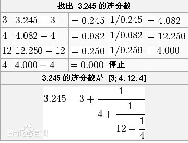
这是一个经典的逼近关系，分数$\frac k d$且$d<φ(N)$在$log_2N$约束内非常逼近$\frac e N$。实际上，所有类似$\frac k d$这样的分数都是$\frac e N$的连分数展开的收敛。因此我们首要做的便是计算$\frac e N$的连分数的$logN$收敛，其中一个连分数就等于$\frac k d$。因为$ed−kφ(N)=1$，我们有$gcd(k,d)=1$，因此$\frac k d$是一个最简分数。这是可以算出密钥d的线性时间算法。

(至于为啥d的上界是那个，别问我，找wiener问去。)

下面是python的代码实现

import gmpy2


def transform(x,y):       #使用辗转相处将分数 x/y 转为连分数的形式
    res=[]
    while y:
        res.append(x//y)
        x,y=y,x%y
    return res
    
def continued_fraction(sub_res):
    numerator,denominator=1,0
    for i in sub_res[::-1]:      #从sublist的后面往前循环
        denominator,numerator=numerator,i*numerator+denominator
    return denominator,numerator   #得到渐进分数的分母和分子，并返回

    
#求解每个渐进分数def sub_fraction(x,y):
    res=transform(x,y)
    res=list(map(continued_fraction,(res[0:i] for i in range(1,len(res)))))  #将连分数的结果逐一截取以求渐进分数
    return res

#以上是获得e/n的连分数

def get_pq(a,b,c):      #由p+q和pq的值通过维达定理来求解p和q
    par=gmpy2.isqrt(b*b-4*a*c)   #由上述可得，开根号一定是整数，因为有解
    x1,x2=(-b+par)//(2*a),(-b-par)//(2*a)
    return x1,x2

def wienerAttack(e,n):
    for (d,k) in sub_fraction(e,n):  #用一个for循环来注意试探e/n的连续函数的渐进分数，直到找到一个满足条件的渐进分数
        if k==0:                     #可能会出现连分数的第一个为0的情况，排除
            continue
        if (e*d-1)%k!=0:             #ed=1 (\pmod φ(n)) 因此如果找到了d的话，(ed-1)会整除φ(n),也就是存在k使得(e*d-1)//k=φ(n)
            continue
        
        phi=(e*d-1)//k               #这个结果就是 φ(n)
        px,qy=get_pq(1,n-phi+1,n)
        if px*qy==n:
            p,q=abs(int(px)),abs(int(qy))     #可能会得到两个负数，负负得正未尝不会出现
            d=gmpy2.invert(e,(p-1)*(q-1))     #求ed=1 (\pmod  φ(n))的结果，也就是e关于 φ(n)的乘法逆元d
            return d
    print("该方法不适用")
    
    
e = 14058695417015334071588010346586749790539913287499707802938898719199384604316115908373997739604466972535533733290829894940306314501336291780396644520926473
n = 33608051123287760315508423639768587307044110783252538766412788814888567164438282747809126528707329215122915093543085008547092423658991866313471837522758159
d = wienerAttack(e,n)
print("d=",d)

Wiener‘s Attack失效时

失效就是意味着界限不满足，而现存的有许多基于Wiener‘s Attack的变型算法就是用来尽量扩大这个界限的。这里是Boneh Durfee Attack的脚本，需要用到多元coppersmith的原理（俺不会，略略略）

利用条件：已知给出n,e,c （e很大） (boneh_durfee.sage)

from __future__ import print_function
import time

############################################
# Config
##########################################

"""
Setting debug to true will display more informations
about the lattice, the bounds, the vectors...
"""
debug = True

"""
Setting strict to true will stop the algorithm (and
return (-1, -1)) if we don't have a correct
upperbound on the determinant. Note that this
doesn't necesseraly mean that no solutions
will be found since the theoretical upperbound is
usualy far away from actual results. That is why
you should probably use `strict = False`
"""
strict = False

"""
This is experimental, but has provided remarkable results
so far. It tries to reduce the lattice as much as it can
while keeping its efficiency. I see no reason not to use
this option, but if things don't work, you should try
disabling it
"""
helpful_only = True
dimension_min = 7 # stop removing if lattice reaches that dimension

############################################
# Functions
##########################################

# display stats on helpful vectors
def helpful_vectors(BB, modulus):
    nothelpful = 0
    for ii in range(BB.dimensions()[0]):
        if BB[ii,ii] >= modulus:
            nothelpful += 1

    print(nothelpful, "/", BB.dimensions()[0], " vectors are not helpful")

# display matrix picture with 0 and X
def matrix_overview(BB, bound):
    for ii in range(BB.dimensions()[0]):
        a = ('%02d ' % ii)
        for jj in range(BB.dimensions()[1]):
            a += '0' if BB[ii,jj] == 0 else 'X'
            if BB.dimensions()[0] < 60:
                a += ' '
        if BB[ii, ii] >= bound:
            a += '~'
        print(a)

# tries to remove unhelpful vectors
# we start at current = n-1 (last vector)
def remove_unhelpful(BB, monomials, bound, current):
    # end of our recursive function
    if current == -1 or BB.dimensions()[0] <= dimension_min:
        return BB

    # we start by checking from the end
    for ii in range(current, -1, -1):
        # if it is unhelpful:
        if BB[ii, ii] >= bound:
            affected_vectors = 0
            affected_vector_index = 0
            # let's check if it affects other vectors
            for jj in range(ii + 1, BB.dimensions()[0]):
                # if another vector is affected:
                # we increase the count
                if BB[jj, ii] != 0:
                    affected_vectors += 1
                    affected_vector_index = jj

            # level:0
            # if no other vectors end up affected
            # we remove it
            if affected_vectors == 0:
                print("* removing unhelpful vector", ii)
                BB = BB.delete_columns([ii])
                BB = BB.delete_rows([ii])
                monomials.pop(ii)
                BB = remove_unhelpful(BB, monomials, bound, ii-1)
                return BB

            # level:1
            # if just one was affected we check
            # if it is affecting someone else
            elif affected_vectors == 1:
                affected_deeper = True
                for kk in range(affected_vector_index + 1, BB.dimensions()[0]):
                    # if it is affecting even one vector
                    # we give up on this one
                    if BB[kk, affected_vector_index] != 0:
                        affected_deeper = False
                # remove both it if no other vector was affected and
                # this helpful vector is not helpful enough
                # compared to our unhelpful one
                if affected_deeper and abs(bound - BB[affected_vector_index, affected_vector_index]) < abs(bound - BB[ii, ii]):
                    print("* removing unhelpful vectors", ii, "and", affected_vector_index)
                    BB = BB.delete_columns([affected_vector_index, ii])
                    BB = BB.delete_rows([affected_vector_index, ii])
                    monomials.pop(affected_vector_index)
                    monomials.pop(ii)
                    BB = remove_unhelpful(BB, monomials, bound, ii-1)
                    return BB
    # nothing happened
    return BB

""" 
Returns:
* 0,0   if it fails
* -1,-1 if `strict=true`, and determinant doesn't bound
* x0,y0 the solutions of `pol`
"""
def boneh_durfee(pol, modulus, mm, tt, XX, YY):
    """
    Boneh and Durfee revisited by Herrmann and May
    
    finds a solution if:
    * d < N^delta
    * |x| < e^delta
    * |y| < e^0.5
    whenever delta < 1 - sqrt(2)/2 ~ 0.292
    """

    # substitution (Herrman and May)
    PR.<u, x, y> = PolynomialRing(ZZ)
    Q = PR.quotient(x*y + 1 - u) # u = xy + 1
    polZ = Q(pol).lift()

    UU = XX*YY + 1

    # x-shifts
    gg = []
    for kk in range(mm + 1):
        for ii in range(mm - kk + 1):
            xshift = x^ii * modulus^(mm - kk) * polZ(u, x, y)^kk
            gg.append(xshift)
    gg.sort()

    # x-shifts list of monomials
    monomials = []
    for polynomial in gg:
        for monomial in polynomial.monomials():
            if monomial not in monomials:
                monomials.append(monomial)
    monomials.sort()
    
    # y-shifts (selected by Herrman and May)
    for jj in range(1, tt + 1):
        for kk in range(floor(mm/tt) * jj, mm + 1):
            yshift = y^jj * polZ(u, x, y)^kk * modulus^(mm - kk)
            yshift = Q(yshift).lift()
            gg.append(yshift) # substitution
    
    # y-shifts list of monomials
    for jj in range(1, tt + 1):
        for kk in range(floor(mm/tt) * jj, mm + 1):
            monomials.append(u^kk * y^jj)

    # construct lattice B
    nn = len(monomials)
    BB = Matrix(ZZ, nn)
    for ii in range(nn):
        BB[ii, 0] = gg[ii](0, 0, 0)
        for jj in range(1, ii + 1):
            if monomials[jj] in gg[ii].monomials():
                BB[ii, jj] = gg[ii].monomial_coefficient(monomials[jj]) * monomials[jj](UU,XX,YY)

    # Prototype to reduce the lattice
    if helpful_only:
        # automatically remove
        BB = remove_unhelpful(BB, monomials, modulus^mm, nn-1)
        # reset dimension
        nn = BB.dimensions()[0]
        if nn == 0:
            print("failure")
            return 0,0

    # check if vectors are helpful
    if debug:
        helpful_vectors(BB, modulus^mm)
    
    # check if determinant is correctly bounded
    det = BB.det()
    bound = modulus^(mm*nn)
    if det >= bound:
        print("We do not have det < bound. Solutions might not be found.")
        print("Try with highers m and t.")
        if debug:
            diff = (log(det) - log(bound)) / log(2)
            print("size det(L) - size e^(m*n) = ", floor(diff))
        if strict:
            return -1, -1
    else:
        print("det(L) < e^(m*n) (good! If a solution exists < N^delta, it will be found)")

    # display the lattice basis
    if debug:
        matrix_overview(BB, modulus^mm)

    # LLL
    if debug:
        print("optimizing basis of the lattice via LLL, this can take a long time")

    BB = BB.LLL()

    if debug:
        print("LLL is done!")

    # transform vector i & j -> polynomials 1 & 2
    if debug:
        print("looking for independent vectors in the lattice")
    found_polynomials = False
    
    for pol1_idx in range(nn - 1):
        for pol2_idx in range(pol1_idx + 1, nn):
            # for i and j, create the two polynomials
            PR.<w,z> = PolynomialRing(ZZ)
            pol1 = pol2 = 0
            for jj in range(nn):
                pol1 += monomials[jj](w*z+1,w,z) * BB[pol1_idx, jj] / monomials[jj](UU,XX,YY)
                pol2 += monomials[jj](w*z+1,w,z) * BB[pol2_idx, jj] / monomials[jj](UU,XX,YY)

            # resultant
            PR.<q> = PolynomialRing(ZZ)
            rr = pol1.resultant(pol2)

            # are these good polynomials?
            if rr.is_zero() or rr.monomials() == [1]:
                continue
            else:
                print("found them, using vectors", pol1_idx, "and", pol2_idx)
                found_polynomials = True
                break
        if found_polynomials:
            break

    if not found_polynomials:
        print("no independant vectors could be found. This should very rarely happen...")
        return 0, 0
    
    rr = rr(q, q)

    # solutions
    soly = rr.roots()

    if len(soly) == 0:
        print("Your prediction (delta) is too small")
        return 0, 0

    soly = soly[0][0]
    ss = pol1(q, soly)
    solx = ss.roots()[0][0]

    #
    return solx, soly

def example():
    ############################################
    # How To Use This Script
    ##########################################

    #
    # The problem to solve (edit the following values)
    #

    # the modulus
    N = 0xc2fd2913bae61f845ac94e4ee1bb10d8531dda830d31bb221dac5f179a8f883f15046d7aa179aff848db2734b8f88cc73d09f35c445c74ee35b01a96eb7b0a6ad9cb9ccd6c02c3f8c55ecabb55501bb2c318a38cac2db69d510e152756054aaed064ac2a454e46d9b3b755b67b46906fbff8dd9aeca6755909333f5f81bf74db
    # the public exponent
    e = 0x19441f679c9609f2484eb9b2658d7138252b847b2ed8ad182be7976ed57a3e441af14897ce041f3e07916445b88181c22f510150584eee4b0f776a5a487a4472a99f2ddc95efdd2b380ab4480533808b8c92e63ace57fb42bac8315fa487d03bec86d854314bc2ec4f99b192bb98710be151599d60f224114f6b33f47e357517

    # the hypothesis on the private exponent (the theoretical maximum is 0.292)
    delta = .18 # this means that d < N^delta

    #
    # Lattice (tweak those values)
    #

    # you should tweak this (after a first run), (e.g. increment it until a solution is found)
    m = 4 # size of the lattice (bigger the better/slower)

    # you need to be a lattice master to tweak these
    t = int((1-2*delta) * m)  # optimization from Herrmann and May
    X = 2*floor(N^delta)  # this _might_ be too much
    Y = floor(N^(1/2))    # correct if p, q are ~ same size

    #
    # Don't touch anything below
    #

    # Problem put in equation
    P.<x,y> = PolynomialRing(ZZ)
    A = int((N+1)/2)
    pol = 1 + x * (A + y)

    #
    # Find the solutions!
    #

    # Checking bounds
    if debug:
        print("=== checking values ===")
        print("* delta:", delta)
        print("* delta < 0.292", delta < 0.292)
        print("* size of e:", int(log(e)/log(2)))
        print("* size of N:", int(log(N)/log(2)))
        print("* m:", m, ", t:", t)

    # boneh_durfee
    if debug:
        print("=== running algorithm ===")
        start_time = time.time()

    solx, soly = boneh_durfee(pol, e, m, t, X, Y)

    # found a solution?
    if solx > 0:
        print("=== solution found ===")
        if False:
            print("x:", solx)
            print("y:", soly)

        d = int(pol(solx, soly) / e)
        print("private key found:", d)
    else:
        print("=== no solution was found ===")

    if debug:
        print(("=== %s seconds ===" % (time.time() - start_time)))

if __name__ == "__main__":
    example()

RSA LSB Oracle Attack

适用情况：可以选择密文发送给服务器，并且服务器返回解密密文后的明文的最低位(LSB)。

在一次RSA加密中，明文为m，模数为n，加密指数为e，密文为c。我们可以构造出$c’\equiv ((2^e)\cdot c) \equiv ((2^e)\cdot (m^e))\equiv ((2\cdot m)^e) \pmod n$， 因为m的两倍可能大于n，所以经过解密得到的明文是 $m’\equiv (2\cdot m)\pmod n$ 。我们还能够知道 m’ 的最低位lsb 是1还是0。 因为n是奇数，而$2\cdot m$是偶数，所以如果lsb 是0，说明$(2\cdot m)%n$ 是偶数，没有超过n，即$m<\frac{n}{2}$，反之则$m>\frac{n}{2}$。

举个例子就能明白2 % 3=2 是偶数，而4 % 3=1 是奇数。以此类推，构造密文$c’’\equiv 4^e\cdot c \pmod n$ 使其解密后为$m’’\equiv (4\cdot m)\pmod n$ ，判断$m’’$ 的奇偶性可以知道m 和 $\frac{n}{4}$ 的大小关系。所以我们就有了一个二分算法，可以在对数时间内将m的范围逼近到一个足够狭窄的空间。

exp:

def get_lsb(c):
    sh.recvuntil(">")
    sh.sendline(str(c))
    rev = sh.recvuntil("\n")[:-1]
    return int(rev)

def oracle(c,n,t):
    L=0
    H=n
    for i in range(1024):
        c = (t*c) % n
        if get_lsb(c) == 0:
            H = (L+H) // 2
        else:
            L = (L+H) // 2
    return long_to_bytes(L)

oracle(c, n, pow(m,2,n))

上面的脚本在最后会出现一些误差，大约一到两个字符，具体原因尚不明确，但是下面这个脚本是没有误差的。

def lsb_oracle_attack(encrypted_flag, n, e):

    flag_count = n_count = 1
    flag_lower_bound = 0
    flag_upper_bound = n
    ciphertext = encrypted_flag
    mult = 1
    while flag_upper_bound > flag_lower_bound + 1:
        ciphertext = (ciphertext * pow(2, e, n)) % n
        flag_count *= 2
        n_count = n_count * 2 - 1
        print("bit = %d" % mult)
        mult += 1
        data=get_lsb(str(ciphertext))
        if(data==1):
            flag_upper_bound = n * n_count / flag_count
        else:
            flag_lower_bound = n * n_count / flag_count
            n_count += 1
    return flag_upper_bound

选择密文攻击

适用情况：可以构造任意密文，服务器会解密密文并返回对应明文。【LSB Oracle Attack的简易版本】

利用RSA的乘法同态性质就好。

这个好理解，在一个RSA加密过程中，明文为m，密文为c，模数为n，加密指数为e，

选取$x$以满足$gcd(x,n) =1$ 从而使$x$模$n$的逆存在，

构造密文$c’ \equiv c\cdot (x^e) \pmod n$使解密后明文为$m’ \equiv (m\cdot x) \pmod n$，

则$m\equiv m’\cdot x^{-1} \pmod n $。

可参看模意义下的运算法则部分。【$x^{-1} = inverse(x,n)$】

RSA经典非预期

这里最后来一个RSA偶尔出现的经典非预期

如果出题人没有设置好明文填充，而是单单把flag作为明文的话，通常情况下这个明文都会比较短，短到$m<p$，（$p$是模数$n$的一个分解）那么我们就可以直接利用$p$作为模数然后正常求解RSA就可以求解得到明文了。2020祥云杯的more_calc这一题就可以直接这样子一把梭。（预期解的原理推起来还挺麻烦的，回头可以记录一下）

至于为啥？$c \equiv m^e \pmod n \rightarrow c \equiv m^e \pmod p$，好推的，自己试试~

Coppersmith相关

移步密码学学习笔记 之 Coppersmith’s Method

---

转载请注明来源，欢迎对文章中的引用来源进行考证，欢迎指出任何有错误或不够清晰的表达。可联系QQ 643713081，也可以邮件至 643713081@qq.com